|
|
The main function to calculate trends and breakpoints on single time series is Trend. This function offers a common access to different methods for trend analysis as assessed in Forkel et al. (2013):
The following methods are tested and compared in this paper based on NDVI time series:
> # load the package and example data
> library(greenbrown)
> data(ndvi) # load the time series
> plot(ndvi) # plot the time series
> # calculate trend (default method: TrendAAT)
> trd <- Trend(ndvi)
> trd
--- Trend ---------------------------------------
Calculate trends and trend changes on time series
-------------------------------------------------
Time series start : 1982 1
Time series end : 2008 1
Time series length : 27
Test for structural change
OLS-based MOSUM test for structural change
statistic : 0.8876267
p-value : 0.2874284
Breakpoints : Breakpoints were not detected.
Trend method : AAT
Trends in segments of the time series
slope % p-value tau
segment 1 : -0.000988 -0.343 0.182 -0.185
> # calculate trend but consider breakpoints
> trd <- Trend(ndvi, mosum.pval=1)
> plot(trd)
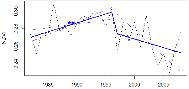
Fig. 1: Trend in mean annual NDVI from an example grid cell in central Alaska.
Other functions exist to calculate non-linear trends on time series based on different methods such as TrendPoly (4th-order polynomial), TrendRunmed (running median), TrendSSA (low frequency component from singular spectrum analysis), TrendSTL (trend component from STL).
The package implements further methods that have been used in Forkel et al. (2013) to estimate properties of NDVI time series and to simulate artificial time series. Statistical properties of time series can be estimated based on the time series decomposition approach as described in Forkel et al. (2013) and implemented in Decompose which is then applied to raster datasets with GetTsStatisticsRaster. SimTs can be used to simulate artificial time series.
The function TrendRaster is used to apply trend and breakpoint estimation methods as implemented in Trend to gridded raster datasets.
> data(ndvimap) # load the example raster data
> ?ndvimap # information about the data
> plot(ndvimap, 8, col=brgr.colors(50))
> # calculate trend on the raster dataset using annual maximum NDVI
> trendmap <- TrendRaster(ndvimap, start=c(1982, 1), freq=12, method="AAT", breaks=1, funAnnual=max)
> plot(trendmap, col=brgr.colors(20), legend.width=2) # this line will produce figure 2:
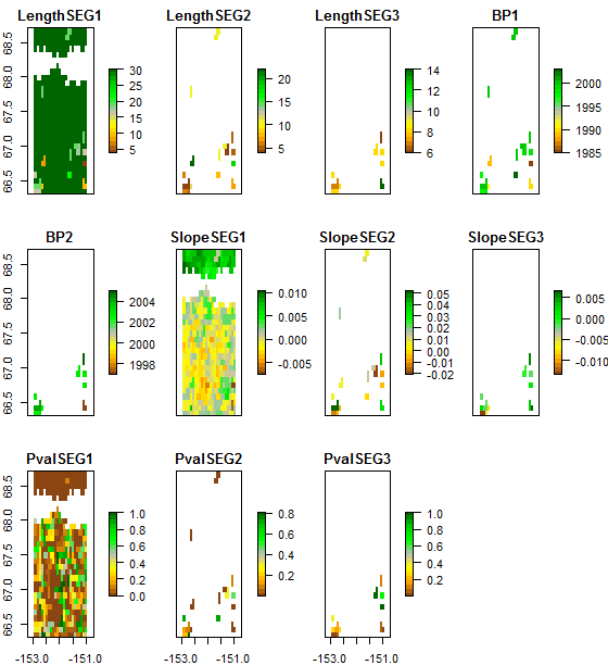
Fig. 2: Trends on annual maximum NDVI with detected breakpoints (BP, year of breakpoint), length of the time series segments (LengthSEG, in years), slope of the trend in each segment (SlopeSEG) and p-value of the trend in each segment (Pval).
Results of this trend and breakpoint analysis can be classified into maps of significant positive or negative trends with TrendClassification.
> trendclassmap <- TrendClassification(trendmap, min.length=8, max.pval=0.05)
> plot(trendclassmap, col=brgr.colors(3), legend.width=2)
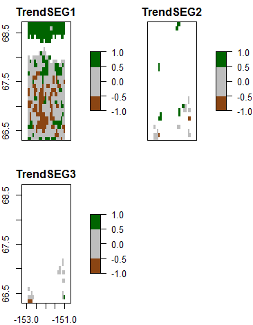
Fig. 3: Significant greening and browning trends on annual maximum NDVI in each time series segment.
The function TrendGradient computes trends along a spatial gradient (e.g. along latitudes). This function extracts along a spatial gradient (e.g. along latitude) time series from a raster brick and computes for each position a temporal trend.
> data(ndvimap)
> # compute a latitudinal gradient of trends (by default the method 'AAT' is used):
> gradient <- TrendGradient(ndvimap, start=c(1982, 1), freq=12)
> plot(gradient)
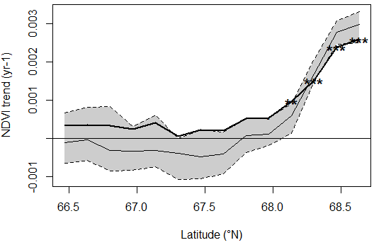
Fig. 4: Latitudinal gradient of NDVI trends. The bold line with significance flags is the estimated trend slope. The gray-colored area and the thin line are the 95% confidence interval and the median, respectively of the estimated trend depending on a sampling of the time series length.
greenbrown offers also some function to compare classifications and maps with classified values. The function AccuracyAssessment computes an accuracy assessment (user accuracy, producer accuracy, total accuracy) from two classifications. CompareClassification compares two classified maps. These functions can be for example used to compare two maps of classified trend (greening/browning/no trend) that were for example calculated with two different methods or from two NDVI data sets.
> data(ndvimap)
> # calculate trends with two different methods
> AATmap <- TrendRaster(ndvimap, start=c(1982, 1), freq=12, method="AAT", breaks=0)
> STMmap <- TrendRaster(ndvimap, start=c(1982, 1), freq=12, method="STM", breaks=0)
> # classify the trend estimates into significant positive, negative and no trend
> AATmap.cl <- TrendClassification(AATmap)
> STMmap.cl <- TrendClassification(STMmap)
> # compare the classified maps
> compare <- CompareClassification(AATmap.cl, STMmap.cl, names=list('AAT'=c("Br", "No", "Gr"), 'STM'=c("Br", "No", "Gr")))
> compare
> # plot the comparison
> plot(compare)
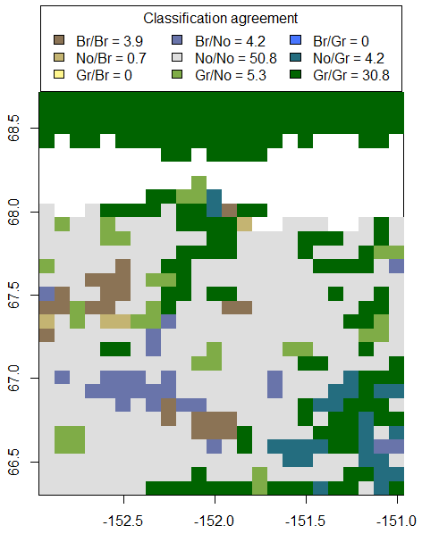
Fig. 5: Comparsion of greening and browning trends on annual mean NDVI from two different methods. Gr/Gr indicates pixels where both maps show greening trends. No cases exist where the two methods have opposite trends (Gr/Br or Br/Gr).
greenbrown, Matthias Forkel, 2016-11-17