greenbrown - land surface phenology and trend analysis

greenbrown: Introduction
Installation and loading
Using greenbrown - applications and examples:

Developer summary page

Using greenbrown: Phenology analysis

Metrics of land surface phenology and greenness are often derived from vegetation index time series to map the spatial variability of vegetation phenology or to analyse temporal changes in vegetation. Phenology and greenness metrics (PGMs) are for example the start and end of growing season (SOS and EOS) or the greenness during the peak of the growing season (PEAK). A description of these metrics and a discussion on the caveats and challenges of phenology detection from remote sensing-derived vegetation index time series can be found in Forkel et al. (2015):

Codominant water control on global interannual variability and trends in land surface phenology and greenness.

In the greenbrown package, phenology detection is implemented as a step-wise procedure with prepocessing and analysis steps as described in Forkel et al. (2015). The steps are:

Filling of permanent gaps in time series
Time series smoothing and interpolation
Detection of phenology events

The corresponding functions to these steps can be used separately or the entire step-wise procedure can be applied just by using the main function Phenology for time series and PhenologyRaster for multi-temporal raster data.

The function Seasonality is used during several steps to check if the time series has seasonality. Otherwise, the calculation of most phenology metrics like SOS and EOS is not useful.

Main functions: Phenology and PhenologyRaster

The main functions for phenology detection that cover these three steps are Phenology for time series and PhenologyRaster for multi-temporal raster data. These two functions encapsulate several other functions that are needed during the different steps and that are explained below.

> # load example NDVI time series
> data(ndvi)
> plot(ndvi)

> # compute phenology metrics
> spl.trs <- Phenology(ndvi, tsgf="TSGFspline", approach="White")
> spl.trs
--- Phenology ----------------------------
Calculate phenology metrics on time series
------------------------------------------

Method
- smoothing and gap filling : TSGFspline
- summary approach : White

Mean and standard deviation of annual metrics:
SOS : 86 +- 11
EOS : 280 +- 15
LOS : 190 +- 21
MSP : 0.27 +- 0.019
MAU : 0.27 +- 0.019
RSP : NaN +- NA
RAU : NaN +- NA
POP : 180 +- 10
POT : 0.37 +- 1.3
MGS : 0.3 +- 0.021
PEAK : 0.32 +- 0.022
TROUGH : 0.23 +- 0.018

> plot(spl.trs)

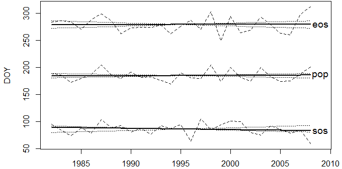
Fig. 1: Annual time series of the the start of growing season (sos), end of growing season (eos) and position of peak day (pop).

The phenology analysis can be easily applied to raster datasets with PhenologyRaster.

> # load example NDVI time series
> data(ndvimap)
> phenmap <- PhenologyRaster(ndvimap, start=c(1982, 1), freq=12, tsgf="TSGFspline", approach="Deriv")
> plot(phenmap, c(grep("SOS.1982", names(phenmap)), grep("EOS.1982", names(phenmap))))

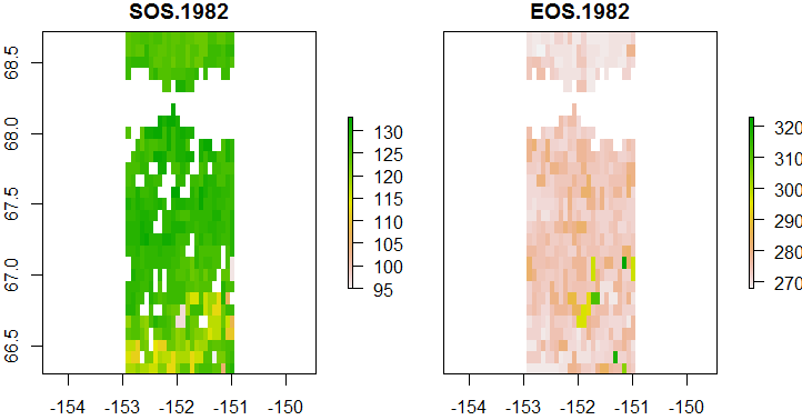
Fig. 2: Maps of start and end of the growing season in 1982 (in day of year).

Step 1 - Filling of permanent gaps in time series: FillPermanentGap

Permanent gaps in time series are missing values that occur regulary every year or in many years. Permanent gaps in satellite-derived vegetation index time series are for example the winter months in northern regions where reliable observation are not possible because of high sun zenit angles or snow cover. Such gaps can be identified using the function IsPermanentGap and these gaps can be filled with FillPermanentGaps.

> data(ndvi)

> # set NA values into winter months to simulate gaps
> winter <- (1:length(ndvi))[cycle(ndvi) == 1 | cycle(ndvi) == 2 | cycle(ndvi) == 12]
> gaps <- sample(winter, length(winter)*0.3)
> ndvi2 <- ndvi
> ndvi2[gaps] <- NA
> plot(ndvi2)

> # check and fill permanent gaps
> IsPermanentGap(ndvi2)
> fill <- FillPermanentGaps(ndvi2) # default fills with the minimum value
> plot(fill, col="red"); lines(ndvi)

Step 2 - Temporal smoothing and gap filling: TsPP

Several functions are implemented to smooth, to gap-fill and interpolate time series to daily time steps:

TSGFlinear: linear interpolation and running median
TSGFspline: spline smoothing and interpolation
TSGFssa: singular spectrum analysis
TSGFdoublelog: fitting of a double-logistic function to the data of each year. Thereby two types of double-logistic function can be currently used: FitDoubleLogBeck and FitDoubleLogElmore

The functions of steps 1 and 2 are both encapsulated by the function TsPP (time series preprocessing).

> data(ndvi)

> # introduce random gaps
> gaps <- ndvi
> gaps[runif(100, 1, length(ndvi))] <- NA

> # smoothing and gap filling
> tsgf <- TSGFspline(gaps)
> plot(gaps, main="Temporal smoothing and gap-filling using splines")
> lines(tsgf, col="red")

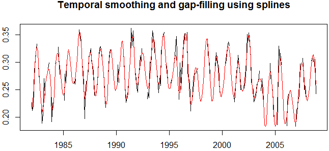
Fig. 3: Original time series with gaps (black) and smoothed and interpolated time series (red).

Step 3 - Detection of phenology events: PhenoDeriv and PhenoTrs

In the last step, phenology events like the start of growing season (SOS) and end of growing season (EOS) are estimated from the daily interpolated, gap-filled and smoothed time series. This can be done either by using thresholds (PhenoTrs) or by extreme values of the derivative of the seasonal cycle (PhenoDeriv). PhenoTrs implements thereby two approaches to estimate phenology events.

> data(ndvi)

> # time series pre-processing
> x <- TsPP(ndvi, interpolate=TRUE)[1:365]

> # calculate phenology metrics for first year
> PhenoDeriv(x, plot=TRUE)

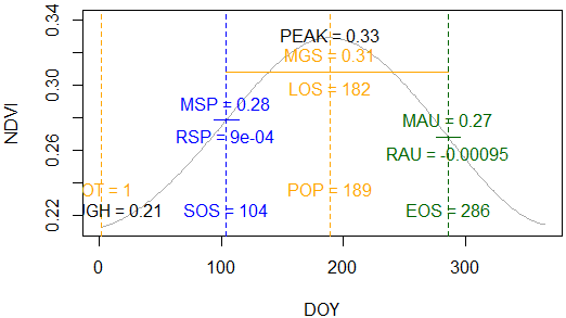
Fig. 4: Seasonal cycle of a single year with estimated PGMs (phenology and greenness metrics).